How to Promote Your ATI Course in Social Media LinkedIn for ATI Rocket Scientists Did you know that for 52% of professionals and executives, their LinkedIn profile is the #1 or #2 search result when someone searches on their name? For ATI instructors, that number is substantially lower – just 17%. One reason is […]
How to Promote Your ATI Course in Social MediaLinkedIn for ATI Rocket Scientists
Did you know that for 52% of professionals and executives, their LinkedIn profile is the #1 or #2 search result when someone searches on their name?
For ATI instructors, that number is substantially lower – just 17%. One reason is that about 25% of ATI instructors do not have a LinkedIn profile. Others have done so little with their profile that it isn’t included in the first page of search results.
If you are not using your LinkedIn profile, you are missing a huge opportunity. When people google you, your LinkedIn profile is likely the first place they go to learn about you. You have little control over what other information might be available on the web about you. But you have complete control over your LinkedIn profile. You can use your profile to tell your story – to give people the exact information you want them to have about your expertise and accomplishments.
Why not take advantage of that to promote your company, your services, and your course?
Here are some simple ways to promote your course using LinkedIn…
On Your LinkedIn Profile
Let’s start by talking about how to include your course on your LinkedIn profile so it is visible anytime someone googles you or visits your profile.
1. Add your role as an instructor.
Let people know that this course is one of the ways you share your knowledge. You can include your role as an instructor in several places on your profile:
Experience – This is the equivalent of listing your role as a current job. (You can have more than one current job.) Use Applied Technology Institute as the employer. Make sure you drag and drop this role below your full-time position.
Summary – Your summary is like a cover letter for your profile – use it to give people an overview of who you are and what you do. You can mention the type of training you do, along with the name of your course.
Projects – The Projects section gives you an excellent way to share the course without giving it the same status as a full-time job.
Headline – Your Headline comes directly below your name, at the top of your profile. You could add “ATI Instructor” at the end of your current Headline.
Start with an introduction, such as “I teach an intensive course through the Applied Technology Institute on [course title]” and copy/paste the description from your course materials or the ATI website. You can add a link to the course description on the ATI website.
This example from Tom Logsdon’s profile, shows how you might phrase it:
Here are some other examples of instructors who include information about their courses on their LinkedIn profile:
Buddy Wellborn – His Headline says “Instructor at ATI” and Buddy includes details about the course in his Experience section.
D. Lee Fugal – Mentions the course in his Summary and Experience.
Jim Jenkins – Courses are included throughout Jim’s profile, including his Headline, Summary, Experience, Projects, and Courses.
2. Link to your course page.
In the Contact Info section of your LinkedIn profile, you can link out to three websites. To add your course, go to Edit Profile, then click on Contact Info (just below your number of connections, next to a Rolodex card icon). Click on the pencil icon to the right of Websites to add a new site.
Choose the type of website you are adding. The best option is “Other:” as that allows you to insert your own name for the link. You have 35 characters – you can use a shortened version of your course title or simply “ATI Course.” Then copy/paste the link to the page about your course.
This example from Jim Jenkins’ profile shows how a customized link looks:
3. Upload course materials.
You can upload course materials to help people better understand the content you cover. You could include PowerPoint presentations (from this course or other training), course handouts (PDFs), videos or graphics. They can be added to your Summary, Experience or Project. You can see an example of an upload above, in Tom Logsdon’s profile.
4. Add skills related to your course.
LinkedIn allows you to include up to 50 skills on your profile. If your current list of skills doesn’t include the topics you cover in your course, you might want to add them.
Go to the Skills & Endorsements section on your Edit Profile page, then click on Add skill. Start typing and let LinkedIn auto-complete your topic. If your exact topic isn’t included in the suggestions, you can add it.
5. Ask students for recommendations.
Are you still in touch with former students who were particularly appreciative of the training you provided in your course? You might want to ask them for a recommendation that you can include on your profile. Here are some tips on asking for recommendations from LinkedIn expert Viveka Von Rosen.
6. Use an exciting background graphic.
You can add an image at the top of your profile – perhaps a photo of you teaching the course, a photo of your course materials, a graphic from your presentation, or simply some images related to your topic. You can see an example on Val Traver’s profile.
Go to Edit Profile, then run your mouse over the top of the page (just above your name). You will see the option to Edit Background. Click there and upload your image. The ideal size is 1400 pixels by 425. LinkedIn prefers a JPG, PNG or GIF. Of course, only upload an image that you have permission to use.
Share News about Your Course
You can also use LinkedIn to attract more attendees to your course every time you teach.
7. When a course date is scheduled, share the news as a status update.
This lets your connections know that you are teaching a course – it’s a great way to reach the people who are most likely to be interested and able to make referrals.
Go to your LinkedIn home page, and click on the box under your photo that says “Share an update.” Copy and paste the URL of the page on the ATI website that has the course description. Once the section below populates with the ATI Courses logo and the course description, delete the URL. Replace it with a comment such as:
“Looking forward to teaching my next course on [title] for @Applied Technology Institute on [date] at [location].”
Note that when you finish typing “@Applied Technology Institute” it will give you the option to click on the company name. When you do that ATI will know you are promoting the course, and will be deeply grateful!
When people comment on your update, it’s nice to like their comment or reply with a “Thank you!” message. Their comment shares the update with their network, so they are giving your course publicity.
If you want to start doing more with status updates, here are some good tips about what to share (and what not to share) from LinkedIn expert Kim Garst.
8. Share the news in LinkedIn Groups.
If you have joined any LinkedIn Groups in your areas of expertise, share the news there too.
Of course, in a Group you want to phrase the message a little differently. Instead of “Looking forward to teaching…” you might say “Registration is now open for…” or “For everyone interested in [topic], I’m teaching…”
You could also ask a thought-provoking question on one of the topics you cover. Here are some tips about how to start an interesting discussion in a LinkedIn Group.
9. Post again if you still have seats available.
If the course date is getting close and you are looking for more people to register, you should post again. The text below will work as a status update and in most LinkedIn Groups.
“We still have several seats open for my course on [title] on [date] at [location]. If you know of anyone who might be interested, could you please forward this? Thanks. ”
“We have had a few last-minute cancellations for my course on [title] on [date] at [location]. Know anyone who might be interested in attending?”
10. Blog about the topic of the course.
When you publish blog posts on LinkedIn using their publishing platform, you get even more exposure than with a status update:
The blog posts are pushed out to all your connections.
They stay visible on your LinkedIn profile, and
They are made available to Google and other search engines.
A blog post published on LinkedIn will rank higher than one posted elsewhere, because LinkedIn is such an authority site. So this can give your course considerable exposure.
You probably have written articles or have other content relevant to the course. Pick something that is 750-1500 words.
To publish it, go to your LinkedIn home page, and click on the link that says “Publish a post.” The interface is very simple – easier than using Microsoft Word. Include an image if you can. You probably have something in your training materials that will be perfect.
At the end of the post, add a sentence that says:
“To learn more, attend my course on [title].”
Link the title to the course description on the ATI website.
For more tips about blogging, you are welcome to join ProResource’s online training website. The How to Write Blog Posts for LinkedIn course is free.
Take the first step
The most important version of your bio in the digital world is your LinkedIn summary. If you only make one change as a result of reading this blog post, it should be to add a strong summary to your LinkedIn profile. Write the summary promoting yourself as an expert in your field, not as a job seeker. Here are some resources that can help:
Write the first draft of your profile in a word processing program to spell-check and ensure you are within the required character counts. Then copy/paste it into the appropriate sections of your LinkedIn profile. You will have a stronger profile that tells your story effectively with just an hour or two of work!
Contributed by guest blogger Judy Schramm. Schramm is the CEO of ProResource, a marketing agency that works with thought leaders to help them create a powerful and effective presence in social media. ProResource offers done-for-you services as well as social media executive coaching. Contact Judy Schramm at jschramm@proresource.com or 703-824-8482.
In June 2014 while on assignment for the Applied Technology Institute in Riva, Maryland, Logsdon and his professional colleague, Dr. Moha El-Ayachi, a professor at Rabat, Morocco, taught a group of international students who were flown into the United Nations Humanitarian Services Center in Brindisi, Italy. The students came in from such far-flung locales as […]
Instructor Tom Logsdon, turquoise shirt at front center, poses with some of his students at the United Nations Humanitarian Center located on the heel of the boot in Brindisi, Italy. Over a period of five days, the students learned how to use the GPS-based radio navigation system to survey their countries with extreme precision. The students and their instructors were flown into Brindisi by the United Nations from various other countries around the globe.
In June 2014 while on assignment for the Applied Technology Institute in Riva, Maryland, Logsdon and his professional colleague, Dr. Moha El-Ayachi, a professor at Rabat, Morocco, taught a group of international students who were flown into the United Nations Humanitarian Services Center in Brindisi, Italy. The students came in from such far-flung locales as Haiti, Liberia, Georgia, Western Sahara, the South Sudan, Germany, and Senegal to learn how to better survey land parcels in their various countries. Studies have shown that if clear, unequivocal boundaries defining property ownership can be assured to the citizens of a Third-World Country, financial prosperity inevitably follows. By mastering modern space-age surveying techniques using Trimble Navigation’s highly precise equipment modules, the international students were able to achieve quarter-inch (1 centimeter) accuracy levels for precise benchmarks situated all over the globe.
This was Logsdon’s second year of teaching the course in Brindisi and the Applied Technology Institute has already been invited to submit bids for another, similar course with the same two instructors for the spring of 2015. The students who converged on Brindisi were all fluent in English and well-versed in American culture. Their special skills were especially helpful to their instructors, Tom and Moha, who trained them to use the precisely timed navigation signals streaming down from the 31 GPS satellites circling the Earth 12,500 miles high.
The DOD’s Request for Proposal for the GPS navigation system was released in 1973.
Rockwell International won that contract to build 12 satellites with the total contract value of $330 million. Over the next dozen years, the company was awarded a total of $3 billion in contracts to build more than 40 GPS navigation satellites. Today 1 billion GPS navigation receivers are serving satisfied users all around the globe. The course taught by Tom and Moha covered a variety of topics of interest to specialized GPS users: What is the GPS? How does it work? What is the best way to build or select a GPS receiver? How is the GPS serving its user base? And how can specialize users find clever new ways accentuate its performance?
The GPS constellation currently consists of 31 satellites. That specialized constellation provides at least six-fold coverage to users everywhere in the world. Each of the GPS satellites transmits precisely timed electromagnetic pulses down to the ground, that require about one 11th of a second to make that quick journey. The electronic circuits inside the GPS receiver measure the signal travel time and multiply it by the speed of light to obtain the line-of-sight range to that particular satellite. When it has made at least four ranging measurements to a comparable number of satellites, the receiver employees a four-dimensional analogy of the Pythagorean theorem to determine its exact position and the exact time. This solution utilizes four equations in four unknowns: the receiver’s three position coordinates and the current time. The GPS system must keep track of time intervals to an astonishing level of precision. A radio wave moving through a vacuum travels a foot in a billionth of a second. So an accurate and effective GPS system must be able to keep track of time to within a few billionths of a second. This is accomplished by designing and building satellite clocks that are so accurate and reliable they would lose or gain only one second every 300,000 years. These amazingly accurate clocks are based on esoteric, but well-understood principles, from quantum mechanics. Despite their amazing accuracy, the clocks on board the GPS satellites must be re-synchronized using hardware modules situated on the ground three times each and every day.
The timing measurements for the GPS system are so accurate and precise Einstein’s two famous Theories of Relativity come into play. The GPS receivers located on or near the ground are in a one-g environment and they are essentially stationary compared the satellites whizzing overhead. A GPS satellite travels around its orbit at a speed of 8600 miles per hour and the gravity at its 12,500-mile altitude above the earth is only six percent as strong as the gravity being experienced by a GPS receiver situated on or near the ground. The difference in speed creates a systematic distortion in time due to Einstein’s Special Theory of Relativity. And the difference in gravitational attraction creates a systematic (and predictable) time distortion due to Einstein’s General Theory Of Relativity. If the designers of the GPS navigation system did not understand and compensate for these relativistic time-dilation effects, the GPS radionavigation system would, on average, be in error by about 7 miles. Fortunately, today’s scientists and engineers have gradually developed a firm grasp of the mathematics associated with relativity so they are able to make extremely accurate compensations to all of the GPS navigation solutions. The positions provided by the GPS, for rapidly moving users such as race cars and military airplanes, are typically accurate to within 15 or 20 feet. For the stationary benchmarks of interest to professional surveyors, the positioning solutions can be accurate to within one quarter of an inch, or about one centimeter.
Tom Logsdon has been teaching short courses for the Applied Technology Institute (www.ATIcourses.com) for more than 20 years. During that interval, he has taught nearly 300 short courses, most of which have spanned 3 to 5 days. His specialties include “Orbital and Launch Mechanics”, “GPS Technology”, “Team-Based Problem Solving”, and “Strapped-Down Inertial Navigation Systems”. Logsdon has written and sold 1.8 million words including 33 nonfiction books. These have included The Robot Revolution (Simon and Schuster), Striking It Rich in Space (Random House), The Navstar Global Positioning System (Van Nostrand Reinhold), Mobile Communications Satellites (McGraw-Hill), and Orbital Mechanics (John Wiley & Sons). All of his books have sold well, but his best-selling work has been Programming in Basic, a college textbook that, over nine printings, has sold 130,000 copies. Logsdon also, on occasion, writes magazine articles and newspaper stories and, over the years, he has written 18,000 words for Encyclopaedia Britannica. In addition, he has applied for a patent, help design an exhibit for the Smithsonian Institution, and helped write the text and design the illustrations for four full-color ads that appeared in the Reader’s Digest.
In 1973 Tom Logsdon received his first assignment on the GPS when he was asked to figure out how many GPS satellites would be required to provide at least fourfold coverage at all times to any receiver located anywhere on planet Earth. What a wonderful assignment for a budding young mathematician! Working in Technicolor— with colored pencils and colored marking pens on oversize quad-pad sheets four times as big as a standard sheet of paper— Logsdon used his hard-won knowledge of three-dimensional geometry, graphical techniques, and integral calculus to puzzle out the salient characteristics of the smallest constellation that would provide the necessary fourfold coverage. He accomplish this in three days— without using any computers! And the constellation he devised was the one that appeared in the winning proposal that brought in $330 million in revenues for Rockwell International.
Even as a young boy growing up wild and free in the Bluegrass Region of Kentucky, Tom Logsdon always seemed to have an intuitive understanding of and subtle mathematical relationships of the type that proved to be so useful in the early days of the American space program. His family had always been “gravel-driveway poor.” At age 18 he had never eaten in a restaurant; he had never stayed in a hotel; he had never visited a museum. But, somehow, he managed to work his way through Eastern Kentucky University as a math-physics major while serving as the office assistant to Dr. Smith Park, head of the mathematics department. He also worked as the editor of the campus newspaper, at a noisy Del Monte Cannery in Markesan, Wisconsin, and as a student trainee at the Naval Ordnance Laboratory in Silver Spring, Maryland.
Later he earned a Master’s Degree in Mathematics from the University of Kentucky where he wrote a regular column for the campus newspaper, played ping-pong with the number 9 competitor in the America, and specialized in a highly abstract branch of mathematics called combinatorial topology. In his 92-page thesis, jam-packed with highly abstract mathematical symbols, he evaluated the connectivity and orientation properties of simplicial and cell complexes and various multidimensional analogies of Veblin’s Theorem.
Soon after he finished his thesis, Logsdon accepted a position as a trajectory and orbital mechanics expert at Douglas Aircraft in Santa Monica, California. His most famous projects there included the giant 135 foot-in-diameter Echo Balloon, the six Transit Navigation Satellites, the Thor-Delta booster, and the third stage of the Saturn V moon rocket. A few years later, he moved on to Rockwell International in Downey, California, where he worked his mathematical magic on the second stage of the Saturn V, the four manned Skylab missions, the 24-satellite constellation of GPS radionavigation satellites, the manned Mars mission of 2016, various unmanned asteroid and comet probes, and the solar-power satellite project which, if it had reached fruition, would have incorporated at least 100 geosynchronous satellites each with a surface area equal to that of Manhattan Island (about 20 square miles).
Among his proudest accomplishments at Rockwell International was the clever utilization of nine different branches of advanced mathematics, in partnership with his friend, Bob Africano, to increase the performance capabilities of the Saturn V moon rocket by 4700 extra pounds of payload bound for the moon — each pound of which was worth five times its weight in 24 karat gold! These important performance gains were accomplished without changing any of the hardware elements on the rocket. Logsdon and Africano, instead, employed their highly specialized knowledge of mathematics and physics to work out ways to operate the mighty Saturn V more efficiently. This involved shaping the trajectories of the rocket for maximum propulsive efficiency, shifting the burning mixture ratio in mid flight in an optimal manner, and analyzing their six-degree-of-freedom post-flight trajectory simulations to minimize the heavy reserve propellants necessary to assure completion of the mission. These powerful breakthroughs in math and physics led to a saving of $3.5 billion for NASA – an amount equal to the lifetime earnings of 2000 average American workers!
Currently, Logsdon and his wife, Cyndy, live in Seal Beach, California. Logsdon is now retired from Rockwell International, but he is still writing books, acting as an expert witness in a variety of aerospace-related legal cases, lecturing professionally at big conventions, and teaching short courses on rocket science, orbital mechanics, and GPS technology at major universities, NASA bases, military installations, and at a variety of international locations. Prior to his recent trips to Italy, Logsdon delivered two lectures at Hong Kong University in southern China and taught two short courses at Stellenbach University near Cape Town, South Africa. Over the past 30 years or so he has taught and lectured at 31 different countries scattered across six continents. At the International Platform Association meetings in Washington, DC, two of his presentations in successive years placed in the top 10 among the 45 professional platform lecturers making presentations there. Colleges and Universities that have sponsored his presentations have included Johns Hopkins, Berkeley, USC, Oxford, North Texas University, the International Space University in Strasbourg, France, Saddleback.
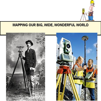
INTRODUCTION Professional surveyors measure, map, and analyze relatively large portions of the Earth’s surface. Armed with precision instruments, they define and record accurate land contours and property boundaries. And they pinpoint the locations of natural landmarks and man-made structures. Surveying has, for centuries, been an essential element of civilized human existence. But it’s practical, everyday […]
INTRODUCTION
Professional surveyors measure, map, and analyze relatively large portions of the Earth’s surface. Armed with precision instruments, they define and record accurate land contours and property boundaries. And they pinpoint the locations of natural landmarks and man-made structures. Surveying has, for centuries, been an essential element of civilized human existence. But it’s practical, everyday im-portance is often overlooked.
Accurate surveying measurements, and the maps that result, make individual property ownership possible. And property ownership, in turn, fosters fruitful human interactions, accentuates the steady accumulation of wealth, and en-hances social prosperity.
“Property is that which is necessary for all civil societies,” observed the famous Scottish philosopher David Hume. America’s 12th president, Abraham Lincoln, echoed a similar sentiment when he concluded that: Property is the fruit of labor . . . It is a positive good in the world. Journalist Leo Rosen was not inclined to contradict President Lincoln’s enthusiastic endorsement. “Property is a sacred trust,” he once concluded, “expressly granted by God, the Bible, and the Recorder’s Office.”
Compelling evidence that property boundaries were being established by sur-veyors as early as 1400 BC has been found among stone carvings found on the broad floodplains and the fertile valleys of ancient Egypt. During the Roman occupation of that prosperous and fertile kingdom, Roman technicians studied, absorbed, and copied the techniques the Egyptians had perfected while they were constructing the great pyramid at Giza.with its nearly perfect proportions and its surprisingly precise north-south alignment.
Around 15 BC, Roman engineers made at least one innovative contribution to the art and science of surveying when they mounted a large, thin wheel in barrel-fashioned on the bottom of a sturdy cart.
When their clever mechanism was pushed along the ground, it automatically dropped a single pebble into a small container with each 360-degree revolution. The number of pebbles rattling around in the container provided a direct measure of the distance traveled by the device. When perfected, it became the world’s first crude, but reliable, odometer!
Roman surveyors refined the methods and mechanisms pioneered by the Egyptians and used their techniques in surveying more than 40,000 miles of Roman roads and in laying out hundreds of miles of aqueducts funneling water to their thirsty cities.
SURVEYING INVENTIONS THAT SPROUTED UP DURING THE RENAISSANCE
In 1620 the famous English mathematician Edmund Gunter develop the earliest surveying chain. It was widely used by surveyors until the steel tape carne into existence 400 years later.
The vernier, a precise auxiliary scale that permitted more accurate readings of dis-tances and angles, was invented in 1631. It was followed by the micrometer micro-scope in 1638 and telescope sights in 1669. The spirit level followed around 1700.A spirit level relies on a small bubble floating in a liquid-filled glass cylinder that is precisely centered when the device is perpendicular the local direction of gravity. .
By the 1920s photogrammetry–the science of constructing accurate maps from aerial photographs–came into general use. And, 50 years later, in the 1970s, orbiting satellites began to serve as dedicated reference points for measuring millions of attitude angles and distances. These measurements allowed contem-porary experts to construct ground-level maps with unprecedented levels of accuracy and convenience. By the 1990s spaceborne centimeter-level surveying had become convenient, practical, and considerably less expensive, too.
Surveying methodologies can be divided into two broad categories: plane surveying – which typically involves distances shorter than 12 miles, and geodetic surveying–which spans areas so large the curvature of the earth must come into play.
PLANE SURVEYING
Plane surveying assumes that the earth is flat in a small local area. Under this con-dition, relatively simple computational algorithms from Euclidean geometry and plane trigonometry can be employed in processing the measurements the surveyor makes. The region being surveyed is typically divided into a small chain of triangles or quadrangles.
When the simpler triangles.are employed, the three interior angles for each tri-angle must sum to 180 degrees and the common side being shared by a pair of the adjacent triangles must be constrained to have the same length in both of the relevant trigonometric calculations. Specialized numerical adjustments force the computations to produce mutually consistent results.
The approach that relies on quadrangles involves four sides, eight angles, and two diagonals. All shared dimensions are forced to end up with mutually consistent results.
GEODETIC SURVEYING ON A MUCH LARGER. SCALE
Geodetic surveying must be applied when the areas being surveyed are so ex-tensive the Earth’s curvature has an appreciable effect on the surveyor’s measurements. In this case spherical trigonometry is required despite the fact that it involves greater complexity and more intricate visualization for those in-terpreting the results.
In 1687 Sir Isaac Newton demonstrated that the earth exhibits a pronounced bulge at the equator. Its first-order spherical shape is distorted by the centrifugal forces induced by its daily rotation.The shape it assumes can be approximated as a oblate spheroid with an equatorial diameter approximately 27 miles longer than its polar diameter.
Huge numbers of measurements affecting the Earth’s non-spherical shape have been incorporated into a variety of mathematical reconstructions of the Earth’s equatorial bulge. These approximations are called datums when they are being used in connection with geodetic surveying.
Leveling measurements establishing a fictitious local sea level are often used in constructing the precise oblate spheroids used in modeling and analyzing surveying operations. One of the earliest and most popular of these models is the Clark ellipsoid of 1866. For more than a century it has been employed as an engineering model defining the shape and gravitational characteristics of our home planet.
Surfaces determined by leveling measurements approximate the average long-term sea level of our home planet. Such surfaces are distorted slightly because, at high northern and southern latitudes, the outer edge of the oblate spheroid is in closer proximity to the Earth’s center where most of its gravity is concentrated.
MODERN ACCOMPLISHMENTS IN AERIAL PHOTOGRAPHY
Military commanders have always struggled to capture and hold the “high ground” because an elevated vantage point often provides an unobstructed view of enemy activities on the ground below. During the American Civil War (circa 1860) hot-air balloons carried reconnaissance experts up among the clouds where they could observe enemy troop deployments and equipment placements.
During World War I and World War II, substantial resources were expended by the various combatants in attempting to survey the sprawling battlefields scattered across continent-wide dimensions. And, when peace ascended over though the smoke-powder battlegrounds, the accuracy and convenience of military surveying and mapmaking operations were appreciably accentuated by aerial observations.
Later in Kentucky (the author’s home state) tobacco acreages were measured, estimated, and controlled by precise government-sponsored surveys of this type. Indeed, this allotment system is still1 .. today, controlled by that same highly efficient approach to terrestrial surveying.
SURVEYING GOD’S GREEN EARTH WITH ORBITING SATELLITES
Orbiting satellites became relatively inaccurate surveying tools shortly after the Rus-sians launched their first Sputnik into outer space in October of 1957. The earliest American satellites used in this manner were the two 100-foot Echo Balloons clearly visible from the surface of the earth. These aluminum-coated mylar balloons allowed crude, but convenient, mapping of otherwise inaccessible regions of the Earth. This could be accomplished by bouncing a sequence of brief radar pulses off the skin of the balloon and timing the bent-pipe signal travel-times between a known location on earth and the one that was yet to be determined.
Camera-equipped satellites have also found widespread applications in surveying and mapmaking enterprises. Shortly after the first Sputnik reached orbit, President Eisenhower presented the ambassador of Brazil with an accurate map of his forest-shrouded country. NASA’s imaging experts had kludged it together by combining dozens of satellite images into a countrywide composite.
Later the six Transit Navigation Satellites and the two dozen or so satellites in the GPS constellation made surveying considerably more accurate, convenient, and cost-effective. GPS-derived sub-centimeter accuracies soon became possible using the precise timing measurements made available by the GPS satellites and their international competitors. Positioning errors were dramatically reduced compared with most conventional surveying techniques. In part, this became possible because ground-based and space-based hardware units and new software modules were soon providing accurate and reliable positioning corrections.
EPILOGUE
Professional surveyors measure, map, and analyze relatively large portions of the Earth’s surface. Armed with precision instruments, they define and record accurate land contours and property boundaries. And they pinpoint the spatial locations of natural landmarks and man-made structures. Surveying has, for many centuries, been an essential element of civilized human existence. But it’s practical, everyday importance is sometimes overlooked.
Hopefully, this brief article will help bring the fundamental importance of pre-cision surveying back into sharp focus.
Tom Logsdon
Seal Beach, California
February, 2015
The Global Positioning System (GPS) was originally designed jointly by the U.S. Navy and the U.S. Air Force to permit the determination of position and time for military troops and guided missiles. However, GPS has also become the basis for position and time measure-ment by scientific laboratories and a wide spectrum of applications in a […]
The Global Positioning System (GPS) was originally designed jointly by the U.S. Navy and the U.S. Air Force to permit the determination of position and time for military troops and guided missiles. However, GPS has also become the basis for position and time measure-ment by scientific laboratories and a wide spectrum of applications in a multi-billion dollar commercial industry. Roughly three billion GPS receivers have been sold to delighted consumers throughout the world. Thirty-one GPS satellites are currently broadcasting navigation signals from their high-altitude vantage points in space.
EARLY METHODS OF NAVIGATION
The shape and size of the earth has been known from the time of antiquity. The fact that the earth is a sphere was well known to educated people as long ago as the fourth century BC. In his book On the Heavens, Aristotle gave two scientifically correct arguments. First, the shad-ow of the earth projected on the moon during a lunar eclipse appears to be curved. Second, the elevations of stars change as one travels north or south, while certain stars visible in Egypt cannot be seen at all from Greece.
The actual radius of the earth was determined within one percent by Eratosthenes in about 230 BC. He knew that the sun was directly overhead at noon on the summer solstice in Syene (Aswan, Egypt), since on that day it illuminated the water of a deep well. At the same time, he measured the length of the shadow cast by a column on the grounds of the library at Alexandria, which was nearly due north. The distance between Alexandria and Syene had been well established by professional runners and camel caravans. Thus Eratosthenes was able to compute the earth’s radius from the difference in latitude that he inferred from his measurement. In terms of modem units of length, he arrived at the figure of about 6400 km. By comparison, the actual mean radius is 6371 km (the earth is not precisely spherical, as the polar radius is 21 km less than the equatorial radius of 6378 km). The ability to determine one’s position on the earth was the next major problem to be addressed. In the second century, AD the Greek astronomer Claudius Ptolemy prepared a geographical atlas, in which he estimated the latitude and longitude of principal cities of the Mediterranean world. Ptolemy is most famous, however, for his geocentric theory of planetary motion, which was the basis for astronomical catalogs until Nicholas Copernicus published his heliocentric theory in 1543.
CELESTIAL NAVIGATION
Historically, methods of navigation over the earth’s surface have involved the angular measure-ment of star positions to determine latitude. The latitude of one’s position is equal to the elevation of the pole star. The position of the pole star on the celestial sphere is only temporary, however, due to precession of the earth’s axis of rotation through a circle of radius 23.5 over a period of 26,000 years. At the time of Julius Caesar, there was no star sufficiently close to the north celes-tial pole to be called a pole star. In 13,000 years, the star Vega will be near the pole. It is perhaps not a coincidence that mariners did not venture far from visible land until the era of Christopher Columbus, when true north could be determined using the star we now call Polaris. Even then the star’s diurnal rotation caused an apparent variation of the compass needle. Polaris in 1492 described a radius of about 3.5 degrees about the celestial pole, compared to today. At sea, however, Columbus and his contemporaries depended primarily on the mariner’s compass and dead reckoning.
The determination of longitude was much more difficult. Longitude is obtained astronomically from the difference between the observed time of a celestial event, such as an eclipse, and the corresponding time tabulated for a reference location. For each hour of difference in time, the difference in longitude is 15 degrees.
NAVIGATION AT SEA
Columbus himself attempted to estimate his longitude on his fourth voyage to the New World by observing the time of a lunar eclipse as seen from the harbor of Santa Gloria in Jamaica on February 29, 1504. In his distinguished biography Admiral of the Ocean Sea, Samuel Eliot Morrison states that Columbus measured the duration of the eclipse with an hour-glass and determined his position as nine hours and fifteen minutes west of Cadiz, Spain, according to the predicted eclipse time in an almanac he carried aboard his ship. Over the preceding year, while his ship was marooned in the harbor, Columbus had determined the latitude of Santa Gloria by numerous observations of the pole star. He made out his latitude to be 18 degrees, which was in error by less than half a degree and was one of the best recorded observations of latitude in the early sixteenth century, but his estimated longitude was off by some 38 degrees.
Columbus also made legendary use of this eclipse by threatening the natives with the disfavor of God, as indicated by a portent from Heaven, if they did not bring desperately needed provisions to his men. When the eclipse arrived as predicted, the natives pleaded for the Admiral’s intervention, promising to furnish all the food that was needed.
New knowledge of the universe was revealed by Galileo Galilei in his book The Starry Messenger. This book, published in Venice in 1610, reported the telescopic discoveries of hundreds of new stars, the craters on the moon, the phases of Venus, the rings of Saturn, sunspots, and the four inner satellites of Jupiter. Galileo suggested using the eclipses of Jupiter’s satellites as a celestial clock for the practical determination of longitude, but the calculation of an accurate ephemeris and the difficulty of observing the satellites from the deck of a rolling ship prevented use of this method at sea. Nevertheless, James Bradley, the third Astronomer Royal of England, successfully applied the technique in 1726 to determine the longitudes of Lisbon and New York with considerable accuracy.
The inability to measure longitude at sea had the potential of catastrophic consequences for sail-ing vessels exploring the new world, carrying cargo, and conquering new territories. Shipwrecks were common. On October 22, 1707 a fleet of twenty-one ships under the command of Admiral Sir Cloudsley Shovel was returning to England after an unsuccessful military attack on Toulon in the Mediterranean. As the fleet approached the English Channel in dense fog, the flagship and three others foundered on the coastal rocks and nearly two thousand men perished.
Stunned by this unprecedented toss, the British government in 1714 offered a prize of 20,000 British Pounds for a method to determine longitude at sea within a half a degree. The scientific establishment believed that the solution would be obtained from observations of the moon.
The German cartographer Tobias Mayer, aided by new mathematical methods developed by Leonard Euler, offered improved tables of the moon in 1757. The recorded position of the moon at a given time as seen from a reference meridian could be compared with its position at the local time to determine the angular position west or east. Just as the astronomical method appeared to achieve realization, the British craftsman John Harrison provided a dif-ferent solution through his invention of the marine chronometer. The story of Harrison’s clock has been recounted in Dava Sobel’s popular book, Longitude.
Both methods were tested by sea trials. The lunar tables permitted the determination of longitude within four minutes of arc, but with Harrison’s chronometer the precision was only one minute of arc. Ultimately, portions of the prize money were awarded to Mayer’s widow, Euler, and Harrison. In the twentieth century, with the development of radio transmitters, another class of navigation aids was created using terrestrial radio beacons, including Loran and Omega. Finally, the tech-nology of artificial satellites made possible navigation and position determination using line of sight signals involving the measurement of Doppler shift or phase difference.
GLOBAL POSITIONING SYSTEM
The success of Transit stimulated both the U.S. Navy and the U.S. Air Force to investigate more advanced versions of a space-based navigation system with enhanced capabilities. Recognizing the need for a combined effort, the Deputy Secretary of Defense established a Joint Program Office in 1973. The NAVSTAR Global Positioning System (GPS) was thus cre-ated.
In contrast to Transit, GPS provides continuous coverage. Also, rather than Doppler shift, satellite range is determined from phase difference. There are two types of observables. One is pseudorange, which is the offset between a pseudorandom noise (PRN) coded signal from the satellite and a replica code generated in the user’s receiver, multiplied by the speed of light. The other is accumulated delta range (ADR), which is a measure of carrier phase.
THE NAVSTAR GPS CONSTELLATION
The original GPS constellation reached operational status in 1995. It consisted of 24 GPS satellites arranged in six orbital rings 10,898 nautical miles above the Earth. Each of the rings was tipped 55 degrees with respect to the equator. More than three billion satisfied users now benefit from the GPS signals streaming down from space.
The determination of position may be described as the process of triangulation using the meas-ured range between the user and four or more satellites. The ranges are inferred from the time of propagation of the satellite signals. Four satellites are required to determine the three co- ordinates of position and time. The time is involved in the correction to the receiver clock and is ultimately eliminated from the measurement of position.
High precision is made possible through the use of atomic clocks carried on-board the satellites. Each satellite has two cesium clocks and two rubidium clocks, which maintain time with a precision one part in ten trillionth in over a few hours, or better than 1O nanoseconds. In terms of the distance traversed by an electromagnetic signal at the speed of light, each nanosecond corresponds to about 30 centimeters. Thus the precision of GPS clocks permits a real time measurement of distance to within a few meters. With post processed carrier phase measurements, a precision of a few centimeters can be achieved today.
The design of the GPS constellation had the fundamental requirement that at least four satellites must be visible at all times from any point on earth. The tradeoffs included visibility, the need to pass over the ground control stations in the United States, cost, and sparing efficiency. The orbital configuration approved in 1973 was a total of 24 satellites, consisting of 8 satellites plus one spare in each of three equally spaced orbital planes. The orbital radius was 26,562 km, corresponding to a period of revolution of 12 sidereal hours, with repeating ground traces. Each satellite arrived over a given point four minutes earlier each day. A common orbital inclination of 63º was selected to maximize the on-orbit payload mass with The operational system, as pres-ently deployed, consists of 21 primary satellites and 3 on-orbit spares, comprising four satellites in each of six orbital planes. Each orbital plane is inclined at 55º with respect to the equator. This constellation improves on the “18 plus 3” satellite constellation by more fully integrating the three active spares.
There have been several generations of GPS satellites. The Block I satellites, built by Rockwell International, were launched between 1978 and 1985. They consisted of eleven prototype satellites, including one launch failure, that validated the system concept. The ten successful satellites had an average lifetime of 8.76 years.
The Block II and Block llA satellites were also built by Rockwell International. Block II consists of nine satellites launched between 1989 and 1990. Block llA, deployed between 1990 and 1997, consists of 19 satellites with several! navigation enhancements. In April 1995, GPS was declared fully operational with a constellation of 24 operational spacecraft and a completed ground segment. The 28 Block II/IIA satellites have exceeded their specified mission duration of 6 years and are expected to have an average lifetime of more than 1O years. Block llR comprises 20 replacement satellites that incorporate autonomous navigation based on cross-link ranging. These satellites are being manufactured by Lockheed Martín. The first launch in 1997 resulted in a launch failure. The first llR satellite to reach orbit was also launched in 1997. The second GPS IIR satellite was successfully launched aboard a Delta 2 rocket on October 7, 1999. One to four more launches are anticipated over the next year. The fourth generation of satellites is the Block II follow-on (Block llF). This program includes the procurement of 33 satellites and the operation and support of a new GPS operational control segment. The Block llF program was awarded to Rockwell (now a part of Boeing). Further details may be found in a special issue of the Proceedings of the IEEE for January, 1999.
CONTROL SEGMENT
The Master Control Station for GPS is located at Schriever Air Force Base in Colorado Springs, CO. The MCS maintains the satellite constellation and performs the station keeping and attitude control maneuvers. It also determines the orbit and clock parameters with a Kalman filter using measurements from five monitor stations distributed around the world. The orbit error is about 1.5 meters.
GPS orbits are derived independently by various scientific organizations using carrier phase and post-processing. The state of the art is exemplified by the work of the International GPS Service (IGS), which produces orbits with an accuracy of approximately 3 centimeters within two weeks. The system time reference is managed by the U.S. Naval Observatory in Washington, DC. GPS time is measured from Saturday/Sunday midnight at the beginning of the week. The GPS time scale is a composite “paper clock” that is synchronized to keep step with Coordinated Universal Time (UTC) and International Atomic Time (TAI). However, UTC differs from TAI by an integral number of leap seconds to maintain correspondence with the rotation of the earth, whereas GPS time does not include leap seconds. The origin of GPS time is midnight on January 5/6, 1980 (UTC). At present, TAI is ahead of UTC by 32 seconds, TAI is ahead of GPS by 19 seconds, and GPS is ahead of UTC by 13 seconds.
Only 1,024 weeks were allotted from the origin before the system time is reset to zero be-cause 1O bits are allocated for the calendar function (1,024 is the tenth power of 2). Thus the first GPS rollover occurred at midnight on August 21, 1999. The next GPS rollover will take place May 25, 2019.
SIGNAL STRUCTURE
The satellite position at any time is computed in the user’s receiver from the navigation message that is contained in a 50 bit per second data stream. The orbit is represented for each one hour period by a set of 15 Keplerian orbital elements, with harmonic coefficients arising from perturbations, and is updated every four hours.
This data stream is modulated by each of two code division multiple access, or spread spectrum, pseudorandom noise (PRN) codes: the coarse/acquisition C/A code (sometimes called the clear/access code) and the precision P code. The P code can be encrypted to produce a secure sig-nal called the Y code. This feature is known as the Anti-Spoof (AS) mode, which is intended to defeat deception jamming by adversaries. The C/A code is used for satellite acquisition and for position determination by civil receivers. The P(Y) code is used by military and other authorized receivers. The C/A code is a Gold code of register size 10, which has a sequence length of 1023 chips and a chipping rate of 1.023 MHz and thus repeats itself every 1 millisecond. (The term “chip” is used instead of “bit’ to indicate that the PRN code contains no information.) The P code is a long code of length 2.3547 x 10¹⁴ chips with a chipping rate of 10 times the C/A code of 10.23 MHz. At this rate the P code has a period of 38.058 weeks, but it is truncated on a weekly basis so that 38 segments are available for the constellation. Each satellite uses a different member of the C/A Gold code family and a different one-week segment of the P code sequence.
The GPS satellites transmit signals at two carrier frequencies: the L1 component with a center frequency of 1575.42 MHz, and the L2 component with a center frequency of 1227.60 MHz. These frequencies are derived from the master clock frequency of 10.23 MHz, with L1 = 154 x 10.23 MHz and L2 = 120 x 10.23 MHz. The L1 frequency transmits both the P code and the C/A code, while the L2 frequency transmits only the P code. The second P code frequency permits a dual-frequency measurement of the ionospheric group delay. The P-code receiver has- a two-sigma root-mean-square horizontal position error of about 5 meters.
The single frequency C/A code user must model the ionospheric delay with less accuracy. In addition, the C/A code is intentionally degraded by a technique called Selective Availability (SA}, which introduces errors of 50 to 100 meters by dithering the satellite clock data.
Through differential GPS measurements, however, position accuracy can be improved by reducing selective availability and environmental errors. The transmitted signal from a GPS satellite has right hand circular polarization. According to the GPS Interface Control Docu-ment, the specified minimum signal strength at an elevation angle of 5 degrees into a linearly polarized receiver antenna with a gain of 3 dB (approximately equivalent to a circularly polarized antenna with a gain of O dB) is – 160 dBW for the L1 C/A code, – 163 dBW far the L1 P code, and – 166 dBW for the L2 P code. The L2 signal is transmitted at a lower power level since it is used primarily for the ionospheric delay correction.
PSEUDORANGE
The fundamental measurement in the Global Positioning System is pseudo- range. The user equipment receives the pseudorandom code from a satellite and, having identified the satellite, generates a replica code. The phase by which the replica code must be shifted in the receiver to maintain maximum correlation with the satellite code, multiplied by the speed of light, is approximately equal to the satellite range. It is called the pseudorange because the measurement must be corrected by a variety of factors to obtain the true range.
The corrections that must be applied include signal propagation delays caused by the ionosphere and the troposphere, the space vehicle clock error, and the user’s receiver clock error. The ionosphere correction is obtained either by measurement of dispersion using the two frequencies L1 and L2 or by calculation from a mathematical model, but the tropospheric delay must be calculated since the troposphere is non dispersive. The true geometric distance to each satellite is obtained by applying these corrections to the measured pseudo- range.
Other error sources and modeling errors continue to be investigated. For example, a recent modification of the Kalman filter has led to improved performance. Studies have also shown that solar radiation pressure models may need revision and there is some new evidence that the earth’s magnetic field may contribute to a small orbit period variation in the satellite clock frequencies.
CARRIER PHASE
Carrier phase is used to performance measurements with a precision that greatly exceeds those based on pseudorange. However, a carrier phase measurement must resolve an integral cycle ambiguity, whereas the pseudorange is unambiguous.
The wavelength of the L1 carrier is about 19 centimeters. Thus with a cycle resolution of one percent, a differential measurement at the level of a few millimeters is theoretically possible. This technique has important applications to geodesy and analogous scientific programs.
RELATIVITY
The precision of GPS measurements is so great that it requires the application of Albert Ein-stein’s special and general theories of relativity for the reduction of its measurements. Professor Carroll Alley of the University of Maryland once articulated the significance of this fact at a scientific conference devoted to time measurement in 1979. He said, “I think it is appropriate to realize that the first practical application of Einstein’s ideas in actual engineering situations are with us in the fact that clocks are now so stable that one must take these small effects into account in a variety of systems that are now undergoing development or are actually in use in comparing time worldwide. It is no longer a matter of scientific interest and scientific application, but it has moved into the realm of engineering necessity.”
According to relativity theory, a moving clock appears to run slow with respect to a similar clock that is at rest. This-effect is called “time dilation.” In addition, a clock in a weaker gravitational potential appears to run fast in comparison to one that is in a stronger gravitational potential. This gravitational effect is known in general as the “red shift” (only in this case it is actually a “blue shift”).
GPS satellites revolve around the earth with a velocity of 3.874 km/s at an altitude of 20, 184 km. Thus on account of the its velocity, a satellite clock appears to run slow by 7 microseconds per day when compared to a clock on the earth’s surface. But on account of the difference in gravitational potential, the satellite clock appears to run fast by 45 microseconds per day. The net effect is that the clock appears to run fast by 38 microseconds per day. This is an enormous rate difference for an atomic clock with a preci-sion of a few nanoseconds. Thus to compensate for this large secular rate, the clocks are given a rate offset prior to satellite launch of – 4.465 parts in 10 to the tenth power from their nominal frequency of 10.23 MHz so that on average they appear to run at the same rate as a clock on the ground. The actual frequency of the satellite clocks before launch is thus 10.22999999543 MHz. Although the GPS satellite orbits are nominally circular, there is al-ways some residual eccentricity. The eccentricity causes the orbit to be slightly elliptical, and the velocity and altitude vary over one revolution. Thus, although the principal velocity and gravitational effects have been compensated by a rate offset, there remains a slight re-sidual variation that is proportional to the eccentricity. For example, with an orbital eccen-tricity of 0.02 there is a relativistic sinusoidal variation in the apparent clock time having an amplitude of 46 nanoseconds. This correction must be calculated and taken into account in the GPS receiver.
The displacement of a receiver on the surface of the earth due to the earth’s rotation in inertial space during the time of flight of the signal must also be taken into account. This is a third relativistic effect that is due to the universality of the speed of light. The maximum correction occurs when the receiver is on the equator and the satellite is on the horizon. The time of flight of a GPS signal from the satellite to a receiver on the earth is then 86 milliseconds and the correction to the range measurement resulting from the receiver displacement is 133 nanoseconds. An analogous correction must be applied by a receiver on a moving platform, such as an aircraft or another satellite. This effect, as interpreted by an observer in the rotating frame of reference of the earth, is called the Sagnac effect. It is also the basis for a laser ring gyro in an inertial navigation system.
GPS MODERNIZATION
In 1996, a Presidential Decision Directive stated the president would review the issue of Selec-tive Availability in 2000 with the objective of discontinuing selective availability no later than 2006. In addition, both the L1 and L2 GPS signals would be made available to civil users and a new civil 10.23 MHz signal would be authorized. To satisfy the needs of aviation, the third civil frequency, known as L5, would be centered at 1176.45 MHz, in the Aeronautical Radio Navigation Services (ARNS) band, subject to approval at the World Radio Conference in 2000. According to Keith McDonald in an article on GPS modernization published in the September, 1999 GPS World, with selective availability removed, the civil GPS accuracy would be improved to about 1O to 30 meters. With the addition of a second frequency for ionospheric group delay corrections, the civil accuracy would become about 5 to 10 meters. A third frequency would permit the creation of two beat frequencies that would yield one-meter accuracy in real time.
A variety of other enhancements are under consideration, including increased power, the addition of a new military code at the L1 and L2 frequencies, additional ground stations, more frequent uploads, and an increase in the number of satellites. These policy initiatives are driven by the dual needs of maintaining national security while supporting the growing dependence on GPS by commercial industry. When these upgrades would begin to be im-plemented in the Block llR and llF satellites depends on GPS funding.
Besides providing position,GPS is a reference for time with an accuracy of 10 nanoseconds or better. Its broadcast time signals are used for national defense, commercial, and scientific purposes. The precision and universal availability of GPS time has produced a paradigm shift in time measurement and dissemination, with GPS evolving from a secondary source to a fundamental reference in itself.
The international community wants assurance that it can rely on the availability of GPS and contin-ued U.S. support for the system. The Russian Global Navigation Satellite System (GLONASS) has been an alternative, but economic conditions in Russia have threatened its continued viability. Consequently, the European Union is considering the creation! of a navigation system of its own, called Galileo, to avoid relying on the U.S. GPS and Russian GLONASS programs.
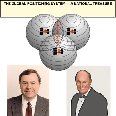
The Global Positioning System is a vital national resource. Over the past thirty years it has made the transition from concept to reality, representing today an operational system on which the entire world has become dependent. Both technical improvements and an enlightened na-tional policy will be necessary to ensure its continued growth into the twenty first century.
Dr. Robert A. Nelson, P.E. was president of Satellite Engineering Research Corporation in Bethesda, Maryland, a Lecturer in the Department of Aerospace Engineering at the University of Maryland and Technical Editor of Via Satellite magazine. Dr. Nelson was the instructor for the ATI course Satellite Communications Systems Engineering for more than 20 years. Dr. Nelson passed away in May 2013. He will be remembered and missed for his many contributions to the field of Satellite Engineering.
Based on an article originally published in Via Satellite. Updated on May 28, 2013 Tom Logsdon has lectured extensively and has taught 300 short courses on a variety of technical topics in 31 different countries scattered across six continents. He as written and sold 1.8 million words in-cluding 32 nonfiction books. His words; spoken and written, have been translated into a dozen different languages including French, Spanish, Serbo-Croatian, Russian, Latvian, Japanese, and International Sign Language. Tom is an expert on GPS and other navigation satellites who teaches several courses for ATlcourses including GPS & Other Radio navigation Satellites , Fundamentals of Orbital & Launch Mechanics, Integrated Navigation Systems , and Introduction to Space.
About Applied Technology Institute Courses (ATlcourses or ATI) ATlcourses is a national leader in professional development seminars in the technical areas of space, communications, defense, sonar, radar,engineering, and signal processing. Since 1984, ATlcourses has presented leading-edge technical training to defense and NASA facilities, as well as DOD and aerospace contractors. ATI courses create a clear understanding of the fundamental principles and a working knowledge of current technology and applications. ATI offers customized on-site training at your facility anywhere in the United States, as well as internationally, and over 200 annual public courses in dozens of locations. ATI is proud to have world-class experts instructing courses. Call 410-956- 8805/888-501-2100, or visit them on the web at www.ATlcourses.com.
By Captain Ray Wellborn, Instructor, Applied Technology Institute On July 4, 2004, the U.S. Navy commissioned the lead ship in a new class of nuclear-powered attack sub-marine: USS VIRGINIA (SSN 774). The new submarine warship is 377 feet in length, 34 feet in the beam, has a draft of 30.5 feet at the designer’s waterline […]
By Captain Ray Wellborn, Instructor,
Applied Technology Institute
On July 4, 2004, the U.S. Navy commissioned the lead ship in a new class of nuclear-powered attack sub-marine: USS VIRGINIA (SSN 774). The new submarine warship is 377 feet in length, 34 feet in the beam, has a draft of 30.5 feet at the designer’s waterline and displaces 7,800 dead weight tons submerged. She can accommodate a ship’s company of 134 including 14 officers.
VIRGINIA’s length-to-breadth ratio of 11.09 is com-parable to an 11.01 for LOS ANGELES-Class submarines with a 33-foot beam, and is somewhat more than SEAWOLF’s 8.4 with a 42-foot beam, but a little less than Ohio’s 13.3, also with a 42-foot beam.
Officially, the U.S. Nary will neither confirm nor deny any U.S. submarine’s speed to be greater than 20 knots, nor any test-depth to be greater than 400 feet.
According to open liter- attire, however, VIRGINIA is powered by a S9G pressurized water reactor, made by General Electric, which will not require re-coring for the life of the ship./ Her propulsion plant is rated to produce 40,000 shaft horsepower for a single shaft, and sustain a maximum rated submerged speed of 34 knots.
The wall-thickness and diameter of VIRGINIA’s inner pressure hull of cold- rolled, high-yield strength steel, with scrupulously designed hull-penetrations and conscientious seam-welds, allows submarine design engineers to impose a safe-diving test-depth of 1,600 feet. Furthermore, this innovative design reduces the number of needed hull-penetrations with eight non-hull penetrating antennae packages.
To meet yet another top-level requirement VIRGINIA is fitted with SEAWOLF-level acoustic quietness for stealth, as well as acoustic tile cladding for active acoustic signal absorption.
For additional tasking, VIRGINIA is fitted with an integral nine-man lockout chamber for use with the Advanced SEAL (sea, air and land) Delivery System (ASDS), which essentially is a mini-submarine capable of dry-delivery of a SEAL team. Moreover, the internal torpedo magazine space arrangement can be adapted to provide 2,400 cubic feet of space for up to 40 SEAL team members arid their equipment. And, VIRGINIA is capable of carrying and operating advanced unmanned underwater vehicles, wake-homing detection equipment and a deployable active hi-static sonar source.
VIRGINIA is an extremely capable submarine and, in the hands of a well- trained, experienced ship’s company skilled in the operational arts of submarine warfare, has an incisive ability for both deep-ocean and shallow- water operations of all kinds, including antisubmarine warfare.
So, for comparison to early strivings for more precise navigation on the open sea, consider the most sophisticated state-of-the art computer-data processors, which precisely calculate the output of an absolutely ingenious arrangement of gyros and accelerometers as they sense the slightest nano-scale movement. This ever-so-precise, self-contained navigational system is fitfully named SINS, the Ship’s Inertial Navigation System. In the modem era, the encapsulated inner workings of SINS can be held in the palm of your hands.
But, at the top of the list, are the technological advancements resident in the Common Submarine Radio Room (CSRR) in that a U.S. submarine can be in constant communication with the submarine operating authority while submerged at sea anywhere in the oceans of the world
For perspective and historical comparison of technological advances, note that the first nationally authorized submarine warship was not officially commissioned until 1900, while the first trans-Atlantic radio-telegraph was not operational until 1901.
VIRGINIA’s modern CSRR for entering the 21st century is for a worldwide battle space. A modernized ship self-defense system will replace the advanced combat direction system in VIRGINIA-Class upgrades.
All the software programs for the command-control system module in VIRGINIA are compatible with the Joint Military Command Information System. The Global Command-Control System (GCCS) is a multi-service information management system for maritime users that displays and disseminates data through an extensive array of common interfaces. GCCS is also a multi-service information management system for maritime users that can display and disseminate data through an extensive array of common interfaces. GCCS is also a multi-sensor data-fusion system for command analyses and decision- making. Thus, in the main, it is utilized for overall force coordination The ocean surveillance information system receives, processes, displays and disseminates joint-service information regarding fixed and mobile targets on land and at sea. The innovative design of the upgraded Automated Digital Network System (ADNS) encompasses all radio frequency circuits for routing and switching both strategic and tactical command control communication computer information (C41) with an internet-like transmission control protocol. In doing so, ADNS links battle group units with each other and with the digital information system network. The ADNS now has 224 ship-based units, and four shore-based sites. Network operation centers are linked to three naval computer and telecommunication area master stations, plus one in the Persian Gulf at Bahrain.
The Global Broadcast Service is the follow-on for U.S. Navy ultra-high- frequency radio communication via satellite. By 2009, the advanced wide- band system will be the communication upgrade for all U.S. submarines and surface ships, and there is a version planned for U.S. aircraft installation that is under study,
Virginia’s combat system suite satisfies a top-level requirement to counter multiple threats with a mission-essential-need statement that details a very effective set of acoustic sensors. The suite features two reel-able towed, linear sonar arrays, the TB-l6 and the thin-line TB-29. Just inside the thin-skinned acoustic window in the bow section of the outer hull is a very sophisticated, state-of-the-art active-passive spherical sonar array, the AN/BQQ-5E.
In addition, there are wide-aperture flank-mounted passive sonar arrays; a keel and fin-mounted high sonic frequency active sonar for under-the-ice ranging and maneuvering, and for mine detection and avoidance; a medium sonic frequency active sonar for target ranging; a sonar sensor for intercept of active-ranging signals from an attacking torpedo; and, a self- noise acoustic monitoring system.
Moreover, all acoustic systems have advanced signal processors and, where appropriate, algorithms are programmed for beam forming.
The Electronic System Measures suite features the AN/BRD-7F radio direction finder; the electronic signal monitors, AN/WLR-lH and AN/WLR-8(V2/6); the AN/WSQ-5 and AN/BLD-1 radio frequency intercept periscope-mounted devices; and the AN/WLQ-4(V1), AN/WLR-l0 and AN/BLQ-l0 radar warning devices. The AN/BPS-15A and BPS-16 are I and J-band navigational piloting radars, respectively, with each having separate wave-guides—one mounted inside a retractable mast and the other mounted inside a periscope.
Virginia has four 21-inch-diameter internally loaded torpedo tubes with storage cradles for a combination of an additional 22 torpedoes, missiles, mines, and 20-foot-long, 21-inch diameter Autonomous Underwater Vehicles.
In the free-flooding area between the outer and inner hulls, just aft of the bow-mounted AN/BQQ-5E spherical sonar array is Virginia’s Vertical Launch System, comprised of twelve externally loaded 21-inch diameter launch tubes for Tomahawk, the Sea-Launched-Cruise-Missile (SLCM).
Shallow water is an anathema for submariners because submarines on the surface are exceptionally vulnerable. Thus, it is said that the best place to sink a submarine is while it is in port. Does that mean that Virginia cannot operate effectively in shallow water?Absolutely not!
Another disconcerting imprecation to submariners is hearing the high-pitch “pings— active sonar accompanied by the shrill of cavitations from small, high-speed screws, which are the distinctive sounds of an acoustic torpedo running to ruin your entire day.
French author Jules Verne (1825-1905) entertained readers with exciting tales of undersea adventure featuring his fictional submarine Nautilus in his book 20,000 Leagues Under The Sea. Notably, USS Nautilus (SSN 571) logged much more than 20,000 leagues under the sea—like, 80,000 nautical mile before her first re-coring, and Virginia will log over 125,000 leagues of submerged steaming in her service life– without refueling.
The nuclear-powered submarine is a far-ranging, very effective, versatile warship for the 21st century—and, the projection of national power by ASDS and SLCMs from international waters only requires unilateral action by the National Command Authority.
U.S. Navy career Captain Ray Wellborn
Over a 30-year U.S. Navy career Captain Ray Wellborn served some 13 years in submarines. He graduated with a B.S. from the U.S. Naval Academy in 1959, a M.S. in Electrical Engineering from the Naval Postgraduate School in 1969, and a M.A. from the Naval War College in 1976. He was a senior lecturer for marine engineering at Texas A&M University Galveston from 1992 to 1996, and currently is a consultant for maritime affairs, and a once-a-year part-time instructor for the Applied Technology Institute’s three-day course titled “Introduction to Submarines—and, Their Combat Systems.
The Global Positioning System A National Resource by Robert A. Nelson On a recent trip to visit the Jet Propulsion Laboratory, I flew from Washington, DC to Los Angeles on a new Boeing 747-400 airplane. The geographical position of the plane and its relation to nearby cities was displayed throughout the flight on a video […]
The Global Positioning System
A National Resource
by Robert A. Nelson
On a recent trip to visit the Jet Propulsion Laboratory, I flew from Washington, DC to Los Angeles on a new Boeing 747-400 airplane. The geographical position of the plane and its relation to nearby cities was displayed throughout the flight on a video screen in the passenger cabin. When I arrived in Los Angeles, I rented a car that was equipped with a navigator. The navigator guided me to my hotel in Pasadena, displaying my position on a map and verbally giving me directions with messages like “freeway exit ahead on the right followed by a left turn.” When I reached the hotel, it announced that I had arrived at my destination. Later, when I was to join a colleague for dinner, I found the restaurant listed in a menu and the navigator took me there.
This remarkable navigation capability is made possible by the Global Positioning System (GPS). It was originally designed jointly by the U.S. Navy and the U.S. Air Force to permit the determination of position and time for military troops and guided missiles. However, GPS has also become the basis for position and time measurement by scientific laboratories and a wide spectrum of applications in a multi-billion dollar commercial industry. Roughly one million receivers are manufactured each year and the total GPS market is expected to approach $ 10 billion by the end of next year. The story of GPS and its principles of measurement are the subjects of this article.
EARLY METHODS OF NAVIGATION
The shape and size of the earth has been known from the time of antiquity. The fact that the earth is a sphere was well known to educated people as long ago as the fourth century BC. In his book On the Heavens, Aristotle gave two scientifically correct arguments. First, the shadow of the earth projected on the moon during a lunar eclipse appears to be curved. Second, the elevations of stars change as one travels north or south, while certain stars visible in Egypt cannot be seen at all from Greece.
The actual radius of the earth was determined within one percent by Eratosthenes in about 230 BC. He knew that the sun was directly overhead at noon on the summer solstice in Syene (Aswan, Egypt), since on that day it illuminated the water of a deep well. At the same time, he measured the length of the shadow cast by a column on the grounds of the library at Alexandria, which was nearly due north. The distance between Alexandria and Syene had been well established by professional runners and camel caravans. Thus Eratosthenes was able to compute the earth’s radius from the difference in latitude that he inferred from his measurement. In terms of modern units of length, he arrived at the figure of about 6400 km. By comparison, the actual mean radius is 6371 km (the earth is not precisely spherical, as the polar radius is 21 km less than the equatorial radius of 6378 km).
The ability to determine one’s position on the earth was the next major problem to be addressed. In the second century, AD the Greek astronomer Claudius Ptolemy prepared a geographical atlas, in which he estimated the latitude and longitude of principal cities of the Mediterranean world. Ptolemy is most famous, however, for his geocentric theory of planetary motion, which was the basis for astronomical catalogs until Nicholas Copernicus published his heliocentric theory in 1543.
Historically, methods of navigation over the earth’s surface have involved the angular measurement of star positions to determine latitude. The latitude of one’s position is equal to the elevation of the pole star. The position of the pole star on the celestial sphere is only temporary, however, due to precession of the earth’s axis of rotation through a circle of radius 23.5 over a period of 26,000 years. At the time of Julius Caesar, there was no star sufficiently close to the north celestial pole to be called a pole star. In 13,000 years, the star Vega will be near the pole. It is perhaps not a coincidence that mariners did not venture far from visible land until the era of Christopher Columbus, when true north could be determined using the star we now call Polaris. Even then the star’s diurnal rotation caused an apparent variation of the compass needle. Polaris in 1492 described a radius of about 3.5 about the celestial pole, compared to 1 today. At sea, however, Columbus and his contemporarie s depended primarily on the mariner’s compass and dead reckoning.
The determination of longitude was much more difficult. Longitude is obtained astronomically from the difference between the observed time of a celestial event, such as an eclipse, and the corresponding time tabulated for a reference location. For each hour of difference in time, the difference in longitude is 15 degrees.
Columbus himself attempted to estimate his longitude on his fourth voyage to the New World by observing the time of a lunar eclipse as seen from the harbor of Santa Gloria in Jamaica on February 29, 1504. In his distinguished biography Admiral of the Ocean Sea, Samuel Eliot Morrison states that Columbus measured the duration of the eclipse with an hour-glass and determined his position as nine hours and fifteen minutes west of Cadiz, Spain, according to the predicted eclipse time in an almanac he carried aboard his ship. Over the preceding year, while his ship was marooned in the harbor, Columbus had determined the latitude of Santa Gloria by numerous observations of the pole star. He made out his latitude to be 18, which was in error by less than half a degree and was one of the best recorded observations of latitude in the early sixteenth century, but his estimated longitude was off by some 38 degrees.
Columbus also made legendary use of this eclipse by threatening the natives with the disfavor of God, as indicated by a portent from Heaven, if they did not bring desperately needed provisions to his men. When the eclipse arrived as predicted, the natives pleaded for the Admiral’s intervention, promising to furnish all the food that was needed.
New knowledge of the universe was revealed by Galileo Galilei in his book The Starry Messenger. This book, published in Venice in 1610, reported the telescopic discoveries of hundreds of new stars, the craters on the moon, the phases of Venus, the rings of Saturn, sunspots, and the four inner satellites of Jupiter. Galileo suggested using the eclipses of Jupiter’s satellites as a celestial clock for the practical determination of longitude, but the calculation of an accurate ephemeris and the difficulty of observing the satellites from the deck of a rolling ship prevented use of this method at sea. Nevertheless, James Bradley, the third Astronomer Royal of England, successfully applied the technique in 1726 to determine the longitudes of Lisbon and New York with considerable accuracy.
Inability to measure longitude at sea had the potential of catastrophic consequences for sailing vessels exploring the new world, carrying cargo, and conquering new territories. Shipwrecks were common. On October 22, 1707 a fleet of twenty-one ships under the command of Admiral Sir Clowdisley Shovell was returning to England after an unsuccessful military attack on Toulon in the Mediterranean. As the fleet approached the English Channel in dense fog, the flagship and three others foundered on the coastal rocks and nearly two thousand men perished.
Stunned by this unprecedented loss, the British government in 1714 offered a prize of £20,000 for a method to determine longitude at sea within a half a degree. The scientific establishment believed that the solution would be obtained from observations of the moon. The German cartographer Tobias Mayer, aided by new mathematical methods developed by Leonard Euler, offered improved tables of the moon in 1757. The recorded position of the moon at a given time as seen from a reference meridian could be compared with its position at the local time to determine the angular position west or east.
Just as the astronomical method appeared to achieve realization, the British craftsman John Harrison provided a different solution through his invention of the marine chronometer. The story of Harrison’s clock has been recounted in Dava Sobel’s popular book, Longitude.
Both methods were tested by sea trials. The lunar tables permitted the determination of longitude within four minutes of arc, but with Harrison’s chronometer the precision was only one minute of arc. Ultimately, portions of the prize money were awarded to Mayer’s widow, Euler, and Harrison.
In the twentieth century, with the development of radio transmitters, another class of navigation aids was created using terrestrial radio beacons, including Loran and Omega. Finally, the technology of artificial satellites made possible navigation and position determination using line of sight signals involving the measurement of Doppler shift or phase difference.
TRANSIT
Transit, the Navy Navigation Satellite System, was conceived in the late 1950s and deployed in the mid-1960s. It was finally retired in 1996 after nearly 33 years of service. The Transit system was developed because of the need to provide accurate navigation data for Polaris missile submarines. As related in an historical perspective by Bradford Parkinson, et al. in the journal Navigation (Spring 1995), the concept was suggested by the predictable but dramatic Doppler frequency shifts from the first Sputnik satellite, launched by the Soviet Union in October, 1957. The Doppler-shifted signals enabled a determination of the orbit using data recorded at one site during a single pass of the satellite. Conversely, if a satellite’s orbit were already known, a radio receiver’s position could be determined from the same Doppler measurements.
The Transit system was composed of six satellites in nearly circular, polar orbits at an altitude of 1075 km. The period of revolution was 107 minutes. The system employed essentially the same Doppler data used to track the Sputnik satellite. However, the orbits of the Transit satellites were precisely determined by tracking them at widely spaced fixed sites. Under favorable conditions, the rms accuracy was 35 to 100 meters. The main problem with Transit was the large gaps in coverage. Users had to interpolate their positions between passes.
GLOBAL POSITIONING SYSTEM
The success of Transit stimulated both the U.S. Navy and the U.S. Air Force to investigate more advanced versions of a space-based navigation system with enhanced capabilities. Recognizing the need for a combined effort, the Deputy Secretary of Defense established a Joint Program Office in 1973. The NAVSTAR Global Positioning System (GPS) was thus created.
In contrast to Transit, GPS provides continuous coverage. Also, rather than Doppler shift, satellite range is determined from phase difference.
There are two types of observables. One is pseudorange, which is the offset between a pseudorandom noise (PRN) coded signal from the satellite and a replica code generated in the user’s receiver, multiplied by the speed of light. The other is accumulated delta range (ADR), which is a measure of carrier phase.
The determination of position may be described as the process of triangulation using the measured range between the user and four or more satellites. The ranges are inferred from the time of propagation of the satellite signals. Four satellites are required to determine the three coordinates of position and time. The time is involved in the correction to the receiver clock and is ultimately eliminated from the measurement of position.
High precision is made possible through the use of atomic clocks carried on-board the satellites. Each satellite has two cesium clocks and two rubidium clocks, which maintain time with a precision of a few parts in 1013 or 1014 over a few hours, or better than 10 nanoseconds. In terms of the distance traversed by an electromagnetic signal at the speed of light, each nanosecond corresponds to about 30 centimeters. Thus the precision of GPS clocks permits a real time measurement of distance to within a few meters. With post-processed carrier phase measurements, a precision of a few centimeters can be achieved.
The design of the GPS constellation had the fundamental requirement that at least four satellites must be visible at all times from any point on earth. The tradeoffs included visibility, the need to pass over the ground control stations in the United States, cost, and sparing efficiency.
The orbital configuration approved in 1973 was a total of 24 satellites, consisting of 8 satellites plus one spare in each of three equally spaced orbital planes. The orbital radius was 26,562 km, corresponding to a period of revolution of 12 sidereal hours, with repeating ground traces. Each satellite arrived over a given point four minutes earlier each day. A common orbital inclination of 63 was selected to maximize the on-orbit payload mass with launches from the Western Test Range. This configuration ensured between 6 and 11 satellites in view at any time.
As envisioned ten years later, the inclination was reduced to 55 and the number of planes was increased to six. The constellation would consist of 18 primary satellites, which represents the absolute minimum number of satellites required to provide continuous global coverage with at least four satellites in view at any point on the earth. In addition, there would be 3 on-orbit spares.
The operational system, as presently deployed, consists of 21 primary satellites and 3 on-orbit spares, comprising four satellites in each of six orbital planes. Each orbital plane is inclined at 55. This constellation improves on the “18 plus 3” satellite constellation by more fully integrating the three active spares.
SPACE SEGMENT
There have been several generations of GPS satellites. The Block I satellites, built by Rockwell International, were launched between 1978 and 1985. They consisted of eleven prototype satellites, including one launch failure, that validated the system concept. The ten successful satellites had an average lifetime of 8.76 years.
The Block II and Block IIA satellites were also built by Rockwell International. Block II consists of nine satellites launched between 1989 and 1990. Block IIA, deployed between 1990 and 1997, consists of 19 satellites with several navigation enhancements. In April 1995, GPS was declared fully operational with a constellation of 24 operational spacecraft and a completed ground segment. The 28 Block II/IIA satellites have exceeded their specified mission duration of 6 years and are expected to have an average lifetime of more than 10 years.
Block IIR comprises 20 replacement satellites that incorporate autonomous navigation based on crosslink ranging. These satellites are being manufactured by Lockheed Martin. The first launch in 1997 resulted in a launch failure. The first IIR satellite to reach orbit was also launched in 1997. The second GPS 2R satellite was successfully launched aboard a Delta 2 rocket on October 7, 1999. One to four more launches are anticipated over the next year.
The fourth generation of satellites is the Block II follow-on (Block IIF). This program includes the procurement of 33 satellites and the operation and support of a new GPS operational control segment. The Block IIF program was awarded to Rockwell (now a part of Boeing). Further details may be found in a special issue of the Proceedings of the IEEE for January, 1999.
CONTROL SEGMENT
The Master Control Station for GPS is located at Schriever Air Force Base in Colorado Springs, CO. The MCS maintains the satellite constellation and performs the stationkeeping and attitude control maneuvers. It also determines the orbit and clock parameters with a Kalman filter using measurements from five monitor stations distributed around the world. The orbit error is about 1.5 meters.
GPS orbits are derived independently by various scientific organizations using carrier phase and post-processing. The state of the art is exemplified by the work of the International GPS Service (IGS), which produces orbits with an accuracy of approximately 3 centimeters within two weeks.
The system time reference is managed by the U.S. Naval Observatory in Washington, DC. GPS time is measured from Saturday/Sunday midnight at the beginning of the week. The GPS time scale is a composite “paper clock” that is synchronized to keep step with Coordinated Universal Time (UTC) and International Atomic Time (TAI). However, UTC differs from TAI by an integral number of leap seconds to maintain correspondence with the rotation of the earth, whereas GPS time does not include leap seconds. The origin of GPS time is midnight on January 5/6, 1980 (UTC). At present, TAI is ahead of UTC by 32 seconds, TAI is ahead of GPS by 19 seconds, and GPS is ahead of UTC by 13 seconds. Only 1,024 weeks were allotted from the origin before the system time is reset to zero because 10 bits are allocated for the calendar function (1,024 is the tenth power of 2). Thus the first GPS rollover occurred at midnight on August 21, 1999. The next GPS rollover will take place May 25, 2019.
SIGNAL STRUCTURE
The satellite position at any time is computed in the user’s receiver from the navigation message that is contained in a 50 bps data stream. The orbit is represented for each one hour period by a set of 15 Keplerian orbital elements, with harmonic coefficients arising from perturbations, and is updated every four hours.
This data stream is modulated by each of two code division multiple access, or spread spectrum, pseudorandom noise (PRN) codes: the coarse/acquisition C/A code (sometimes called the clear/access code) and the precision P code. The P code can be encrypted to produce a secure signal called the Y code. This feature is known as the Anti-Spoof (AS) mode, which is intended to defeat deception jamming by adversaries. The C/A code is used for satellite acquisition and for position determination by civil receivers. The P(Y) code is used by military and other authorized receivers.
The C/A code is a Gold code of register size 10, which has a sequence length of 1023 chips and a chipping rate of 1.023 MHz and thus repeats itself every 1 millisecond. (The term “chip” is used instead of “bit” to indicate that the PRN code contains no information.) The P code is a long code of length 2.3547 x 10¹⁴ chips with a chipping rate of 10 times the C/A code, or 10.23 MHz. At this rate, the P code has a period of 38.058 weeks, but it is truncated on a weekly basis so that 38 segments are available for the constellation. Each satellite uses a different member of the C/A Gold code family and a different one-week segment of the P code sequence.
The GPS satellites transmit signals at two carrier frequencies: the L1 component with a center frequency of 1575.42 MHz, and the L2 component with a center frequency of 1227.60 MHz. These frequencies are derived from the master clock frequency of 10.23 MHz, with L1 = 154 x 10.23 MHz and L2 = 120 x 10.23 MHz. The L1 frequency transmits both the P code and the C/A code, while the L2 frequency transmits only the P code. The second P code frequency permits a dual-frequency measurement of the ionospheric group delay. The P-code receiver has a two-sigma rms horizontal position error of about 5 meters.
The single frequency C/A code user must model the ionospheric delay with less accuracy. In addition, the C/A code is intentionally degraded by a technique called Selective Availability (SA), which introduces errors of 50 to 100 meters by dithering the satellite clock data. Through differential GPS measurements, however, position accuracy can be improved by reducing SA and environmental errors.
The transmitted signal from a GPS satellite has right hand circular polarization. According to the GPS Interface Control Document, the specified minimum signal strength at an elevation angle of 5 into a linearly polarized receiver antenna with a gain of 3 dB (approximately equivalent to a circularly polarized antenna with a gain of 0 dB) is – 160 dBW for the L1 C/A code, – 163 dBW for the L1 P code, and – 166 dBW for the L2 P code. The L2 signal is transmitted at a lower power level since it is used primarily for the ionospheric delay correction.
PSEUDORANGE
The fundamental measurement in the Global Positioning System is pseudorange. The user equipment receives the PRN code from a satellite and, having identified the satellite, generates a replica code. The phase by which the replica code must be shifted in the receiver to maintain maximum correlation with the satellite code, multiplied by the speed of light, is approximately equal to the satellite range. It is called the pseudorange because the measurement must be corrected by a variety of factors to obtain the true range.
The corrections that must be applied include signal propagation delays caused by the ionosphere and the troposphere, the space vehicle clock error, and the user’s receiver clock error. The ionosphere correction is obtained either by measurement of dispersion using the two frequencies L1 and L2 or by calculation from a mathematical model, but the tropospheric delay must be calculated since the troposphere is nondispersive. The true geometric distance to each satellite is obtained by applying these corrections to the measured pseudorange.
Other error sources and modeling errors continue to be investigated. For example, a recent modification of the Kalman filter has led to improved performance. Studies have also shown that solar radiation pressure models may need revision and there is some new evidence that the earth’s magnetic field may contribute to a small orbit period variation in the satellite clock frequencies.
CARRIER PHASE
Carrier phase is used to perform measurements with a precision that greatly exceeds those based on pseudorange. However, a carrier phase measurement must resolve an integral cycle ambiguity whereas the pseudorange is unambiguous.
The wavelength of the L1 carrier is about 19 centimeters. Thus with a cycle resolution of one percent, a differential measurement at the level of a few millimeters is theoretically possible. This technique has important applications to geodesy and analogous scientific programs.
RELATIVITY
The precision of GPS measurements is so great that it requires the application of Albert Einstein’s special and general theories of relativity for the reduction of its measurements. Professor Carroll Alley of the University of Maryland once articulated the significance of this fact at a scientific conference devoted to time measurement in 1979. He said, “I think it is appropriate … to realize that the first practical application of Einstein’s ideas in actual engineering situations are with us in the fact that clocks are now so stable that one must take these small effects into account in a variety of systems that are now undergoing development or are actually in use in comparing time worldwide. It is no longer a matter of scientific interest and scientific application, but it has moved into the realm of engineering necessity.”
According to relativity theory, a moving clock appears to run slow with respect to a similar clock that is at rest. This effect is called “time dilation.” In addition, a clock in a weaker gravitational potential appears to run fast in comparison to one that is in a stronger gravitational potential. This gravitational effect is known in general as the “red shift” (only in this case it is actually a “blue shift”).
GPS satellites revolve around the earth with a velocity of 3.874 km/s at an altitude of 20,184 km. Thus on account of the its velocity, a satellite clock appears to run slow by 7 microseconds per day when compared to a clock on the earth’s surface. But on account of the difference in gravitational potential, the satellite clock appears to run fast by 45 microseconds per day. The net effect is that the clock appears to run fast by 38 microseconds per day. This is an enormous rate difference for an atomic clock with a precision of a few nanoseconds. Thus to compensate for this large secular rate, the clocks are given a rate offset prior to satellite launch of – 4.465 parts in 1010 from their nominal frequency of 10.23 MHz so that on average they appear to run at the same rate as a clock on the ground. The actual frequency of the satellite clocks before launch is thus 10.22999999543 MHz.
Although the GPS satellite orbits are nominally circular, there is always some residual eccentricity. The eccentricity causes the orbit to be slightly elliptical, and the velocity and altitude vary over one revolution. Thus, although the principal velocity and gravitational effects have been compensated by a rate offset, there remains a slight residual variation that is proportional to the eccentricity. For example, with an orbital eccentricity of 0.02 there is a relativistic sinusoidal variation in the apparent clock time having an amplitude of 46 nanoseconds. This correction must be calculated and taken into account in the GPS receiver.
The displacement of a receiver on the surface of the earth due to the earth’s rotation in inertial space during the time of flight of the signal must also be taken into account. This is a third relativistic effect that is due to the universality of the speed of light. The maximum correction occurs when the receiver is on the equator and the satellite is on the horizon. The time of flight of a GPS signal from the satellite to a receiver on the earth is then 86 milliseconds and the correction to the range measurement resulting from the receiver displacement is 133 nanoseconds. An analogous correction must be applied by a receiver on a moving platform, such as an aircraft or another satellite. This effect, as interpreted by an observer in the rotating frame of reference of the earth, is called the Sagnac effect. It is also the basis for a laser ring gyro in an inertial navigation system.
GPS MODERNIZATION
In 1996, a Presidential Decision Directive stated the president would review the issue of Selective Availability in 2000 with the objective of discontinuing SA no later than 2006. In addition, both the L1 and L2 GPS signals would be made available to civil users and a new civil 10.23 MHz signal would be authorized. To satisfy the needs of aviation, the third civil frequency, known as L5, would be centered at 1176.45 MHz, in the Aeronautical Radio Navigation Services (ARNS) band, subject to approval at the World Radio Conference in 2000. According to Keith McDonald in an article on GPS modernization published in the September, 1999 GPS World, with SA removed the civil GPS accuracy would be improved to about 10 to 30 meters. With the addition of a second frequency for ionospheric group delay corrections, the civil accuracy would become about 5 to 10 meters. A third frequency would permit the creation of two beat frequencies that would yield one-meter accuracy in real time.
A variety of other enhancements are under consideration, including increased power, the addition of a new military code at the L1 and L2 frequencies, additional ground stations, more frequent uploads, and an increase in the number of satellites. These policy initiatives are driven by the dual needs of maintaining national security while supporting the growing dependence on GPS by commercial industry. When these upgrades would begin to be implemented in the Block IIR and IIF satellites depends on GPS funding.
Besides providing position, GPS is a reference for time with an accuracy of 10 nanoseconds or better. Its broadcast time signals are used for national defense, commercial, and scientific purposes. The precision and universal availability of GPS time has produced a paradigm shift in time measurement and dissemination, with GPS evolving from a secondary source to a fundamental reference in itself.
The international community wants assurance that it can rely on the availability of GPS and continued U.S. support for the system. The Russian Global Navigation Satellite System (GLONASS) has been an alternative, but economic conditions in Russia have threatened its continued viability. Consequently, the European Union is considering the creation of a navigation system of its own, called Galileo, to avoide relying on the U.S. GPS and Russian GLONASS programs.
The Global Positioning System is a vital national resource. Over the past thirty years it has made the transition from concept to reality, representing today an operational system on which the entire world has become dependent. Both technical improvements and an enlightened national policy will be necessary to ensure its continued growth into the twenty-first century.
____________________________________________
Dr. Robert A. Nelson, P.E. is president of Satellite Engineering Research Corporation, a satellite engineering consulting firm in Bethesda, Maryland, a Lecturer in the Department of Aerospace Engineering at the University of Maryland and Technical Editor of Via Satellite magazine. Dr. Nelson is the instructor for the ATI course Satellite Communications Systems Engineering. Please see our Schedule for dates and locations.
 How to Promote Your ATI Course in Social Media
LinkedIn for ATI Rocket Scientists
Did you know that for 52% of professionals and executives, their LinkedIn profile is the #1 or #2 search result when someone searches on their name?
For ATI instructors, that number is substantially lower – just 17%. One reason is that about 25% of ATI instructors do not have a LinkedIn profile. Others have done so little with their profile that it isn’t included in the first page of search results.
If you are not using your LinkedIn profile, you are missing a huge opportunity. When people google you, your LinkedIn profile is likely the first place they go to learn about you. You have little control over what other information might be available on the web about you. But you have complete control over your LinkedIn profile. You can use your profile to tell your story – to give people the exact information you want them to have about your expertise and accomplishments.
Why not take advantage of that to promote your company, your services, and your course?
How to Promote Your ATI Course in Social Media
LinkedIn for ATI Rocket Scientists
Did you know that for 52% of professionals and executives, their LinkedIn profile is the #1 or #2 search result when someone searches on their name?
For ATI instructors, that number is substantially lower – just 17%. One reason is that about 25% of ATI instructors do not have a LinkedIn profile. Others have done so little with their profile that it isn’t included in the first page of search results.
If you are not using your LinkedIn profile, you are missing a huge opportunity. When people google you, your LinkedIn profile is likely the first place they go to learn about you. You have little control over what other information might be available on the web about you. But you have complete control over your LinkedIn profile. You can use your profile to tell your story – to give people the exact information you want them to have about your expertise and accomplishments.
Why not take advantage of that to promote your company, your services, and your course?
 Here are some simple ways to promote your course using LinkedIn…
On Your LinkedIn Profile
Let’s start by talking about how to include your course on your LinkedIn profile so it is visible anytime someone googles you or visits your profile.
1. Add your role as an instructor.
Let people know that this course is one of the ways you share your knowledge. You can include your role as an instructor in several places on your profile:
Here are some simple ways to promote your course using LinkedIn…
On Your LinkedIn Profile
Let’s start by talking about how to include your course on your LinkedIn profile so it is visible anytime someone googles you or visits your profile.
1. Add your role as an instructor.
Let people know that this course is one of the ways you share your knowledge. You can include your role as an instructor in several places on your profile:
 3. Upload course materials.
You can upload course materials to help people better understand the content you cover. You could include PowerPoint presentations (from this course or other training), course handouts (PDFs), videos or graphics. They can be added to your Summary, Experience or Project. You can see an example of an upload above, in Tom Logsdon’s profile.
4. Add skills related to your course.
LinkedIn allows you to include up to 50 skills on your profile. If your current list of skills doesn’t include the topics you cover in your course, you might want to add them.
Go to the Skills & Endorsements section on your Edit Profile page, then click on Add skill. Start typing and let LinkedIn auto-complete your topic. If your exact topic isn’t included in the suggestions, you can add it.
5. Ask students for recommendations.
Are you still in touch with former students who were particularly appreciative of the training you provided in your course? You might want to ask them for a recommendation that you can include on your profile. Here are some tips on asking for recommendations from LinkedIn expert Viveka Von Rosen.
6. Use an exciting background graphic.
You can add an image at the top of your profile – perhaps a photo of you teaching the course, a photo of your course materials, a graphic from your presentation, or simply some images related to your topic. You can see an example on Val Traver’s profile.
Go to Edit Profile, then run your mouse over the top of the page (just above your name). You will see the option to Edit Background. Click there and upload your image. The ideal size is 1400 pixels by 425. LinkedIn prefers a JPG, PNG or GIF. Of course, only upload an image that you have permission to use.
Share News about Your Course
You can also use LinkedIn to attract more attendees to your course every time you teach.
7. When a course date is scheduled, share the news as a status update.
This lets your connections know that you are teaching a course – it’s a great way to reach the people who are most likely to be interested and able to make referrals.
Go to your LinkedIn home page, and click on the box under your photo that says “Share an update.” Copy and paste the URL of the page on the ATI website that has the course description. Once the section below populates with the ATI Courses logo and the course description, delete the URL. Replace it with a comment such as:
“Looking forward to teaching my next course on [title] for @Applied Technology Institute on [date] at [location].”
Note that when you finish typing “@Applied Technology Institute” it will give you the option to click on the company name. When you do that ATI will know you are promoting the course, and will be deeply grateful!
When people comment on your update, it’s nice to like their comment or reply with a “Thank you!” message. Their comment shares the update with their network, so they are giving your course publicity.
If you want to start doing more with status updates, here are some good tips about what to share (and what not to share) from LinkedIn expert Kim Garst.
8. Share the news in LinkedIn Groups.
If you have joined any LinkedIn Groups in your areas of expertise, share the news there too.
Of course, in a Group you want to phrase the message a little differently. Instead of “Looking forward to teaching…” you might say “Registration is now open for…” or “For everyone interested in [topic], I’m teaching…”
You could also ask a thought-provoking question on one of the topics you cover. Here are some tips about how to start an interesting discussion in a LinkedIn Group.
9. Post again if you still have seats available.
If the course date is getting close and you are looking for more people to register, you should post again. The text below will work as a status update and in most LinkedIn Groups.
“We still have several seats open for my course on [title] on [date] at [location]. If you know of anyone who might be interested, could you please forward this? Thanks. ”
“We have had a few last-minute cancellations for my course on [title] on [date] at [location]. Know anyone who might be interested in attending?”
10. Blog about the topic of the course.
When you publish blog posts on LinkedIn using their publishing platform, you get even more exposure than with a status update:
3. Upload course materials.
You can upload course materials to help people better understand the content you cover. You could include PowerPoint presentations (from this course or other training), course handouts (PDFs), videos or graphics. They can be added to your Summary, Experience or Project. You can see an example of an upload above, in Tom Logsdon’s profile.
4. Add skills related to your course.
LinkedIn allows you to include up to 50 skills on your profile. If your current list of skills doesn’t include the topics you cover in your course, you might want to add them.
Go to the Skills & Endorsements section on your Edit Profile page, then click on Add skill. Start typing and let LinkedIn auto-complete your topic. If your exact topic isn’t included in the suggestions, you can add it.
5. Ask students for recommendations.
Are you still in touch with former students who were particularly appreciative of the training you provided in your course? You might want to ask them for a recommendation that you can include on your profile. Here are some tips on asking for recommendations from LinkedIn expert Viveka Von Rosen.
6. Use an exciting background graphic.
You can add an image at the top of your profile – perhaps a photo of you teaching the course, a photo of your course materials, a graphic from your presentation, or simply some images related to your topic. You can see an example on Val Traver’s profile.
Go to Edit Profile, then run your mouse over the top of the page (just above your name). You will see the option to Edit Background. Click there and upload your image. The ideal size is 1400 pixels by 425. LinkedIn prefers a JPG, PNG or GIF. Of course, only upload an image that you have permission to use.
Share News about Your Course
You can also use LinkedIn to attract more attendees to your course every time you teach.
7. When a course date is scheduled, share the news as a status update.
This lets your connections know that you are teaching a course – it’s a great way to reach the people who are most likely to be interested and able to make referrals.
Go to your LinkedIn home page, and click on the box under your photo that says “Share an update.” Copy and paste the URL of the page on the ATI website that has the course description. Once the section below populates with the ATI Courses logo and the course description, delete the URL. Replace it with a comment such as:
“Looking forward to teaching my next course on [title] for @Applied Technology Institute on [date] at [location].”
Note that when you finish typing “@Applied Technology Institute” it will give you the option to click on the company name. When you do that ATI will know you are promoting the course, and will be deeply grateful!
When people comment on your update, it’s nice to like their comment or reply with a “Thank you!” message. Their comment shares the update with their network, so they are giving your course publicity.
If you want to start doing more with status updates, here are some good tips about what to share (and what not to share) from LinkedIn expert Kim Garst.
8. Share the news in LinkedIn Groups.
If you have joined any LinkedIn Groups in your areas of expertise, share the news there too.
Of course, in a Group you want to phrase the message a little differently. Instead of “Looking forward to teaching…” you might say “Registration is now open for…” or “For everyone interested in [topic], I’m teaching…”
You could also ask a thought-provoking question on one of the topics you cover. Here are some tips about how to start an interesting discussion in a LinkedIn Group.
9. Post again if you still have seats available.
If the course date is getting close and you are looking for more people to register, you should post again. The text below will work as a status update and in most LinkedIn Groups.
“We still have several seats open for my course on [title] on [date] at [location]. If you know of anyone who might be interested, could you please forward this? Thanks. ”
“We have had a few last-minute cancellations for my course on [title] on [date] at [location]. Know anyone who might be interested in attending?”
10. Blog about the topic of the course.
When you publish blog posts on LinkedIn using their publishing platform, you get even more exposure than with a status update: